WFM Goals
Contents
New WFM Goals
The future WFM standard outlines both traditional goals and new goals to address the changing dynamics described the drivers behind the need for change, with special emphasis on “uncertainty”.
Traditional contact center goals which are applied to workforce management normally include service level achievement and budget/expense management. WFM teams can heavily influence both service level and expenses in the range of processes they manage. Naturally, achieving service level and expense can be expected to be two goals WFM teams can be partially accountable for.
Extending from the desire to deliver service level while optimizing expenses, common goals directly tied to WFM organizations include:
- Forecast Accuracy (Volume)
- Schedule Quality Index
- Mean Time to Respond/Repair for Intraday Variance
Organizations may choose to track forecast accuracy on the handling time, shrinkage, and occupancy.
What currently is uncommon is an emphasis on goal setting for forecasting the supply, or employee counts. Most WFM organizations trend attrition, but do not extend models to predict whether employees will stay or go. Incorporated in the new processes is the need to design correlation and causation methods to better understand which employees are likely to remain, which are likely to leave, and begin speaking to “Forecasting Attrition” in the same fashion as WFM forecasts call volume.
New: Forecast Accuracy: Attrition/Retention
A new goal presented in the future WFM standard tracks employee attrition (or the inverse, employee retention rates) to further highlight the significant impact employee turnover has on contact center organizations. Traditionally, WFM teams have trended employee attrition, but far less frequently has it been the mission of WFM to seek correlations and causation drivers which lead to increases or decreases in employee attrition rates.
The future WFM standard seeks to set goals for predicting attrition or retention rates; seeking out drivers, studying correlations and testing hypotheses which predict rates of change. While countless factors influence employee attrition, by assigning an accuracy metric to the variable, we facilitate conversation around the drivers, raising the importance of these input in our capacity planning. This standard will also leverage a cost-calculation methodology for pricing the costs associated with attrition, a value often underestimated.
New: Probability & Variance Goals
A second goal presented in the future WFM standard assigns probability variables within capacity models. This standard then seeks to assign the goal of forecasting a variable accurately by assigning upper & lower limits to represent how wide a variance is likely behind the forecasted model input. Addressing variance is critical to introducing resilient, risk assessed forecasts, and as such, these variance ranges should become a part of goal setting.
Incorporating variance planning into our future model involves challenging a commonly used tactic in WFM: Optimizing to "net zero" ahead of time. By optimizing to net zero, we establish the forecasted required FTEs for a given time period, and schedule enough staff to be "right sized". By doing so, traditional WFM practices create capacity plans which are thought of as fragile - the smallest variance in the wrong direction (demand exceeding supply) quickly impacts service level, customer experience and agent experience in a negative manner.
By introducing variance factors into our processes & goal setting, forecast accuracy can be viewed in a probabilistic fashion facilitating the assignment of risk-ratings and advocating for more resilient capacity plans.
Forecast Accuracy Goals: Call Volume
For decades, much has been published on mathematical methods geared toward time-series forecasting and forecast accuracy. Forecast accuracy has long been a concern of senior management, especially when missing either service level objectives or expense targets. “How accurate was our forecast?” has been heard by all WFM leaders, as if the lack of accuracy would provide an excuse (or scapegoat) for why contact center objectives were missed.
The new WFM standard maintains that forecast accuracy is important goal & metric to establish and leverage continuously. Only by reflecting on how accurate our forecasts are can we drive conversation and ask “why?” a model was off. The critical outcome behind leveraging forecast accuracy is to facilitate uncovering drivers behind any variable which can contribute to the overall completeness of our forecast.
This standard recommends establishing a forecast accuracy metric, at minimum on call volume, and incorporating some concepts in determining how to establish the metric. Questions to ask in establishing a forecast accuracy target:
- What is the queue size you are forecasting for? A queue that delivers 12 million calls annually will have a tighter forecast accuracy target than a queue delivering 1.2 million calls annually.
- What are your hours of operation? Contact centers which are open 8 hours a day, 5 days a week will have a tighter forecast accuracy target than the same call volume delivered over a 24-hour, 7 day a week operation.
- What type of business drivers can be exposed that have predictable correlations? In certain industries, call volumes can be closely tied with predictable events, such as a marketing mailer. Other industries may use subscriber data, policy holder data or other customer counts to correlate to a predictable inquiry rate. Furthermore, some industries have predictable contact rate with seasonality, such as the travel industry, but can suffer in forecast accuracy from non-predictable events, such as storms.
- What is your historical track record for forecast accuracy? While you may not be satisfied by simply trending average forecast accuracy and establishing this as a goal, it is useful to look at the performance of various forecasters in establishing or adjusting forecast accuracy goals.
- What time horizons do you wish to examine forecast accuracy, interval, daily, weekly, monthly, annually? Each time horizon should be monitored for accuracy, but you will likely want to establish a goal on one time horizon rather than many time horizons. Often, teams will focus on a daily accuracy goal, as WFM software cares for distributing the call volume down to the interval level.
This standard does not recommend following the often-publicized advice of “+/-5 percent accuracy as the industry standard”. No such standard exists, nor should it, given the wide range of variables contributing to any team’s ability to forecast accurately, and the nature of variability across differing time horizons.
This standard does recommend queue size as the leading indicator for establishing your forecast accuracy goals, and further recommends leveraging the weighted absolute percentage error (WAPE) method for tracking forecast accuracy.
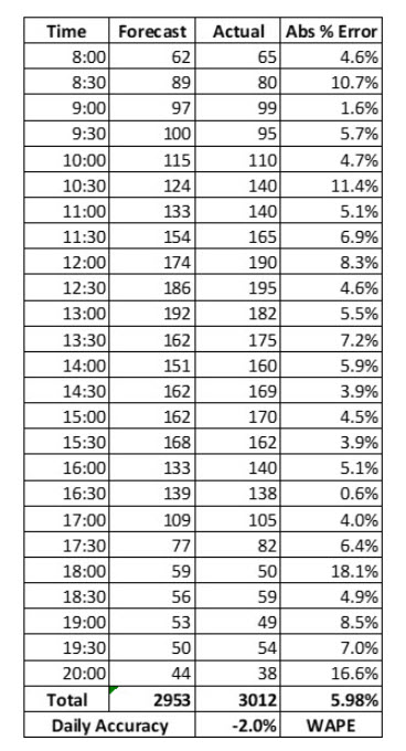
Examining the WAPE method, we presented a day where 2,952 calls were forecasted across a time horizon lasting from 8:00AM to 8:00PM:
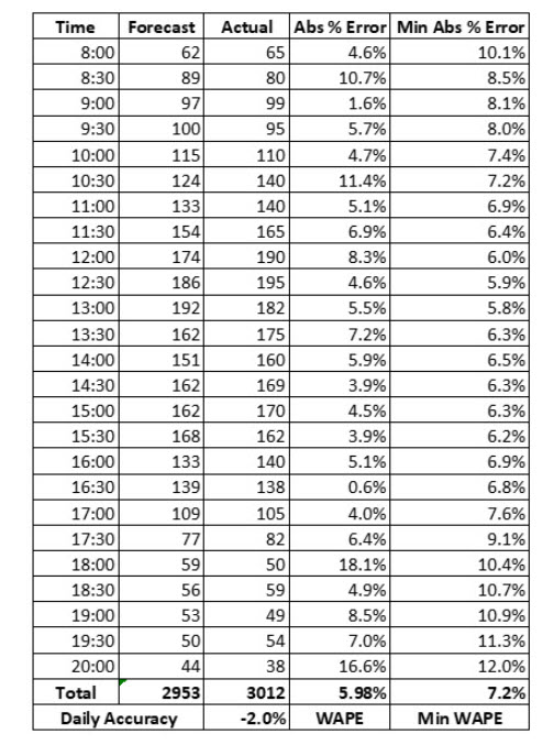
In the above example, each absolute interval variance is calculated, with a weighted absolute percentage error of 5.98% total. When we compare the pure error rate for the day, we see we forecast 2953 against an actual of 3012, or -2.0%. Whether we think this is good or not begins at the interval level, and can be examined by using the following formula, which represents the minimum absolute error rate:
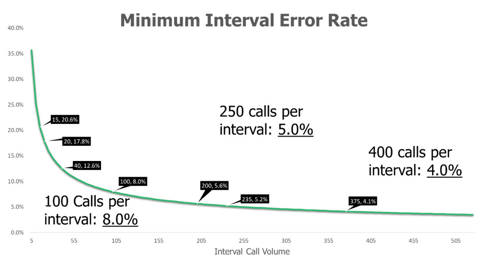
Using the formula to calculate the minimal absolute error rate, we get a sense of the degree of natural error that can not be “forecasted away” through any means. This is a natural intraday variance that can and should be expected when we establish goals and is discussed later in resilient capacity planning. The formula can easily be leveraged to plot a minimum interval variance rate based on the call volume forecasted for any interval.
This provides simple logic to debunk the fact that there could be a unified “industry standard” behind forecast accuracy – the minimal variance factor alone shows that this isn’t practical given that queue groups vary in size and arrival patterns fluctuate.
Schedule Quality Index Goals
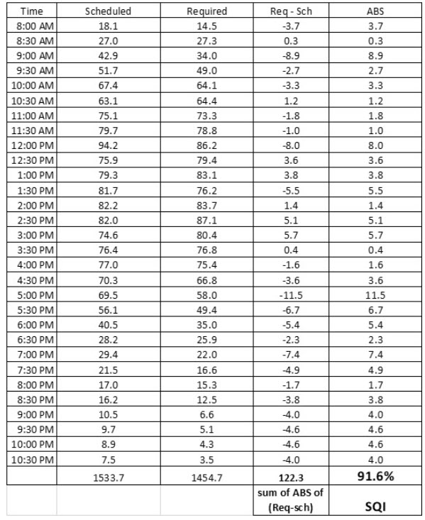
Schedule Quality Index (SQI) allows a WFM organization to measure how tight agent schedules fit the forecast arrival pattern. The calculation can be leveraged as a goal, but it is important to this goal is balanced against the employee-first approach to the next generation WFM model.
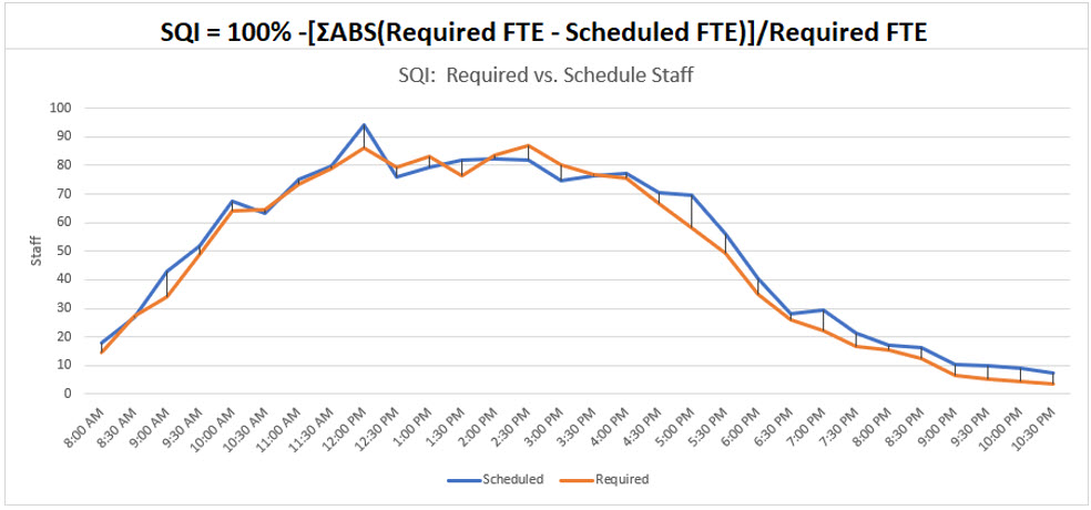
The SQI formula simply looks at the sum of the gaps between agents scheduled and agents required, and expressing those gaps as a % of how far our staffing is off from the forecasted required FTE by interval. The metric than takes 1 - % of gaps to calculate the metric, where 100% would represent an absolute perfect fit. By understanding the percentage gap, decisions can be made as to designing new tour patterns, conducting shift-bids, or ensuring proper automation techniques are in place to close these gaps. A sample calculation:
Where 91.6% SQI = 100% - (Absolute value (122.3/1454.7)
Like forecast accuracy, no industry standard target for this goal exists. Rather, the metric will vary depending on queue groups size, and as important, schedule policy for types of tours designed and shift-bidding principles. In the traditional WFM model, an organization would attempt to drive SQI higher by conducting shift bids and creating a variety of tour types to simulate schedule fit. In the future workforce management model, it is recommended that the goal be tracked, but that employee retention be dimensioned against tour design, and that automation be leveraged to close SQI gaps.
Mean Time to Respond/Repair for Intraday Variance
Real-time teams generally leverage “response rates” to intraday incidents or action submitted for execution. Mean Time to Repair is a traditional metric leveraged in command center environments which seek to measure how quickly teams fix or respond to a scenario where a service or system is down or degraded. Having a goal for turn-around time with a real-time team is useful to set expectations and prioritizations with the team members responding to issues. It is also effective in communicating with stakeholder customers and demonstrating how well the real-time team is performing against service level agreements in place.
MTTR results are normally dimensioned against service level agreements, which may have levels of severity to set expectations:
Within the WFM process section, we will examine how automations can be leveraged to remove the need for real-time teams to respond/repair types of events. In adopting automation techniques for responding, overall goals established for MTTR may require review.
Forecast Accuracy – Attrition / Retention Goal
The future WFM standard seeks to highlight the importance of predicting how many people will be staffed to service the needs of our customers. Be establishing either an employee attrition (or retention) goal, we highlight the importance of this variable. When a goal is set, and we highlight how good (or bad) we are at achieving that goal, we drive conversation and study of a wider range of people variables. Are we spending adequate time coaching and training employees? Are employees being over-worked? Are employees being regularly recognized? These questions sound like the domain of the contact center management, or perhaps HR, or your learning & development department. But workforce management teams are in a unique position; WFM teams forecast a wide range of variables, critical to ensuring we’re set up for achieving financial and customer experience goals.
By taking the same processes leveraged to forecast other variables like call volume, handle time, shrinkage, and occupancy, the future WFM standard adds forecasting attrition/retention percentages and establishing a target goal for the accuracy of predicting this metric.
The method outlined in the future WFM model tracks weekly forecast vs. actual on staffing:
- Starting Staff
- Hires
- Exits
- Available Staff
… and compares the forecasted attrition % against the actual attrition percentage to generate a forecast attrition error %. On a weekly basis, this error rate would be calculated, and then annualized, and presented with the annualized forecasted attrition percentage, and actual attrition percentage:
The section seeks further feedback and input from WFM community.Share spreadsheet for calculation methodology & validation w/ community.
Probability & Variance Goals
In Forecast Accuracy Goals: Call Volume - we speak to the importance of maintaining forecast accuracy goals against metrics such as volume. By reflecting on how accurate our forecasts were, we drive critical conversations which uncover and address the drivers behind why a forecast was off. Yet, single point capacity plan inputs and outputs ignore the important nature our data – capacity plans aggregate variables. Variables change within the context of our capacity plans, and describing how these variables have a distribution of values, is key to enabling resilient capacity planning.
The future WFM standard seeks to directly incorporate variance ranges into the planning cycle and establish the initial goal of conducting simulations to demonstrate the importance variance plays in evaluating risks associated with the capacity plans. These goals can then be expanded to establish target goals for the distribution ranges themselves.
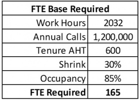
The legacy approach in capacity planning took input variables and sought to assign single-point outcomes. Leveraging a simple base FTE required calculation (not including turnover factors and speed to proficiency) – we calculate:
FTE Required = Annual Calls X AHT /3600 / Work Hours / Occupancy / (1-Shrink):
This assumes no variance to our plan, and that we will need precisely 165 FTE to service the workload. Of course, there is little to no chance that our inputs will line up precisely; we accept that these are continuous variables that will take on a range of values. Yet, the legacy WFM capacity planning approach generally does not formalize a process to incorporate those ranges into our planning cycles.
The future WFM standard seeks to establish the goal of assigning ranges into our planning process by describing the distribution of these variables and conducting simulations (see process section X.X) to determine the probabilistic distribution of outcomes (FTE required, budget). The standard further seeks to expose how the inputs influence these outcome ranges.
The simple FTE required model described above is enhanced to acknowledge that each of these inputs (except for work hours) has a range of outcomes:
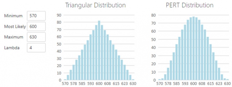
And with that range of outcomes, you have a range of FTEs potentially required. Further, this range can be described by the distribution type assigned, such as AHT with a target of 600 seconds. With the triangular distribution and the PERT distribution, we see probabilities take shape based on the nature of their distribution density:
Establishing the goal of assigning ranges to variables in capacity planning facilitates the next section, establishing risk ratings.Risk Ratings
The section seeks further feedback and input from WFM community.
In a risk assessment, variance refers to the degree of uncertainty or unpredictability associated with a particular risk. The higher the variance, the greater the uncertainty and the more difficult it is to predict the likelihood and impact of a risk.
In general, higher variance implies higher risk, as there is a greater range of potential outcomes and a greater uncertainty about which outcome will occur. For example, if a risk has a high variance, it may be difficult to predict how likely it is to occur or how severe the consequences might be. This can make it difficult to effectively plan for and manage the risk.
On the other hand, a risk with low variance is more predictable and easier to plan for. For example, if a risk has a low variance, it may be more likely to occur, and the consequences may be more predictable and easier to mitigate.
In a risk assessment, it is important to consider the variance associated with a particular risk in order to accurately assess and manage the risk. This can help to identify strategies for mitigating or eliminating the risk, as well as to establish contingency plans in case the risk does materialize.
By introducing variance planning and variance goals associated with establishing variance ranges (rather than single-point outcomes), the future workforce operating model seeks to establish a qualitative risk rating system, one which leverages a consistent quantitative framework. This system would leverage structured ranges that focus on:
- Service Level Risk: The relationship between staffing levels set in the budget, and probabilities of achieving service level based on the variance distributions,
- Financial Risk: The relationship between the staffing levels set in the budget, and the corresponding budget allocated to service the capacity model,
- Employee Risk: The relationship between occupancy levels set, productive shrink investment, attrition rates, and the probability to deliver against the each (future development)
- Overall Risk: A combination of service level risk, financial risk, and employee risk to generate an overall rating.
Service Level Risk Rating
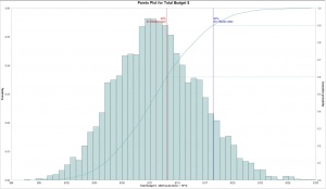
The service level risk rating assumes variance planning is in place, and that the WFM team has presented a representative distribution of values associated each variable feeding the capacity model. Those inputs can then generate a range of staffing requirements with a plot representing what % of outcomes would be covered, based on the staffing levels established.
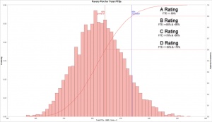
When the range of inputs is run through a Monte Carlo simulation, an output histogram / Pareto can be examined. By segmenting the % of scenarios covered across the Pareto range, one can then translate the final FTE set in the budget against the % of outcomes that staffing level covers. Ranges could be communicated as:
- FTE >= 90% receives an A Rating,
- FTE >=80% & <90% receives a B Rating
- FTE >=70% & <80% receives a C Rating
- FTE >=60% & <70% receives a D Rating
... and so on, aligning to a traditional qualitative rating system.
Financial Risk Rating
Relative to how a financial department works with the data presented by workforce management, every organization treats capacity planning slightly different. In some cases, finance may dictate a target budget expense, independent of the staffing models presented. In far fewer cases, the finance department may incorporate the staffing plan the WFM team develops, establishing the budget from the recommended capacity plan outputs. In most organizations, the process lies between these two extremes, where finance and workforce management may go through multiple iterative rounds to land on a final staffing / expense value, with each round negotiating & justifying "why volume, handle time, shrink, occupancy, and attrition is X% higher or lower than last year"
To assign a qualitative risk score to the final budget value, we consider that it is less likely organizations operate purely on a "service level-first" model at any cost. If your organization simply staffs to any value presented, then assigning a financial risk rating has little meaning in this system; you would simply give your Service Level an "A" and if fully funded, Financial risk would be minimal (an A-Rating) so long as your capacity plan projections were sound.
Given that finance generally has a strong hand in many organizations, we'll assume for this risk rating system that there will be a gap between the desired WFM staffing levels generated with the FTE distribution, and the associated financial budget being allocated to staff the contact center. Within this approach, assigning a risk rating, or likelihood to achieve budget requires we take a true risk-assessed FTE distribution, and examine the ability to tune our staffing levels down when staffing variances run positive (FTE actual > FTE required at any point in time).
Key points to stress before assigning financial risk rating:
- The capacity plan should not incorporate unproven bets. Example, in an initial round of modeling, AHT for tenured agents runs 600 seconds, with a minimum value of 570 and a maximum value 630, and the distribution is forecasted leveraging a PERT distribution described above. If in a subsequent round of planning, AHT is lowered to 580 with no corresponding reasoning (we'll just find a way to hit that number), then the associated risk rating system becomes invalid.
- The capacity plan should assume right-sized staffing at the start of a planning cycle. Entering a planning cycle short-staffed introduces instability into operations and again invalidates the logic leveraged to assign a risk rating.
To establish the financial risk rating, we examine the outputs of both our FTE distribution and the associated financial distributions charts. In a simple grid, we align the FTEs required to staff a plan with the associated SL risk ratings as such:
| FTE | SL Risk | Budget | ||
| 233.8 | A | $ 11,788,284 | or more | |
| 229.8 | 233.7 | B | $ 11,580,815 | $ 11,788,283 |
| 226.9 | 229.7 | C | $ 11,415,519 | $ 11,580,814 |
| 224.5 | 226.8 | D | $ 11,284,090 | $ 11,415,518 |
| 224.4 | F | less than | $ 11,284,089 | |
In that a plan with 234 FTE would receive an "A Rating" against service level. We also see that this plan would translate into a budget of ~$11.8 million. As we indicated, rarely does finance wish to cover all possible outcomes and simply assign the associated budget. For this exercise, we assume finance assigns a budget of $11.225 million, presenting a budget gap, assuming we plan to staff to 234:
| FTE | SL Risk | Budget | Budget Gap | ||
| 233.8 | A | $ 11,788,284 | or more | $ (563,284) | |
| 229.8 | 233.7 | B | $ 11,580,815 | $ 11,788,283 | $ (355,815) |
| 226.9 | 229.7 | C | $ 11,415,519 | $ 11,580,814 | $ (190,519) |
| 224.5 | 226.8 | D | $ 11,284,090 | $ 11,415,518 | $ (59,090) |
| 224.4 | F | less than | $ 11,284,089 | ||
| Budget | $ 11,225,000 | ||||
| Planned Staff | 234 | ||||
If we are positioned to be adequately staffed to 234 FTE, we have a budget gap of $563k, or approximately 5%. While our scenarios modeled leveraging Monte Carlo simulation indicate 243 FTE would cover 90% of outcomes, that staff hedges to the right of the curve of the outcomes. To assess our financial risk, we introduce the degree to which we can remove costs consistently leveraging automation. These methods are a key enabler in the future WFM operating model; staffing above the mean, and leveraging natural variability plus automation to optimize service level and expense.
To generate a financial risk assumption, we categorize what real-time automations are in place & adoption rates to forecast the expense to be removed
| Automation Adoption | High | Medium | Low | None |
| VTO | $ 117,882.84 | $ 70,729.70 | ||
| Training | $ 259,342.25 | $ 212,189.11 | $ 165,035.98 | |
| Coaching | $ 141,459.41 | |||
| AHT/ACW | $ 58,941.42 | $ 23,576.57 | $ 11,788.28 | |
| Adherence | $ 7,072.97 | $ 5,894.14 | ||
| Total Automations | $ 584,698.89 | $ 312,389.53 | $ 176,824.26 | $ - |
| Adjusted Gap | $ 21,414.89 | $ (250,894.47) | $ (386,459.74) | $ (563,284.00) |
| % Gap Budget | 0.2% | -2.2% | -3.4% | -5.0% |
| Meet | Miss by 2.2% | Miss by 3.4% | Miss by 5% |
Then the results are combined with the organization's threshold for budget achievement, example:
| Budget | Financial Risk |
| Meet or Exceed | A |
| Miss by up to 3% | B |
| Miss by 4%-5% | C |
| Miss 6-7% | D |
| Miss >7% | F |
In the above example, the FTE staffed was 234, however, automation reduced expenses in the high adoption category to meet budget.
Employee Risk Rating
The relationship between occupancy levels set, productive shrink investment, attrition rates, and the probability to deliver against the each (future development).
Overall Risk Rating
Currently, a combination of: Service Level Risk + Financial Risk as described above.
